
Derivation of the counterflow effectiveness-NTU relation
Target Audience: Engineers or engineering students who've got some understanding of Calculus and Thermo.
In order to really grasp some engineering concepts, I need to derive them myself, in a way that makes sense to me. One of these concepts is the ε-NTU method for counterflow heat exchangers.
The final result that relates a counterflow heat exchanger's effectiveness with \(N_{tu}\) (or NTU) for those who haven't seen it before is:
\[ \epsilon = \frac{1 - e^{-NTU(1-\frac{C_{min}}{C_{max}})}}{1 - \frac{C_{min}}{C_{max}} e^{-NTU(1 - \frac{C_min{}}{C_{max}} )}} \]
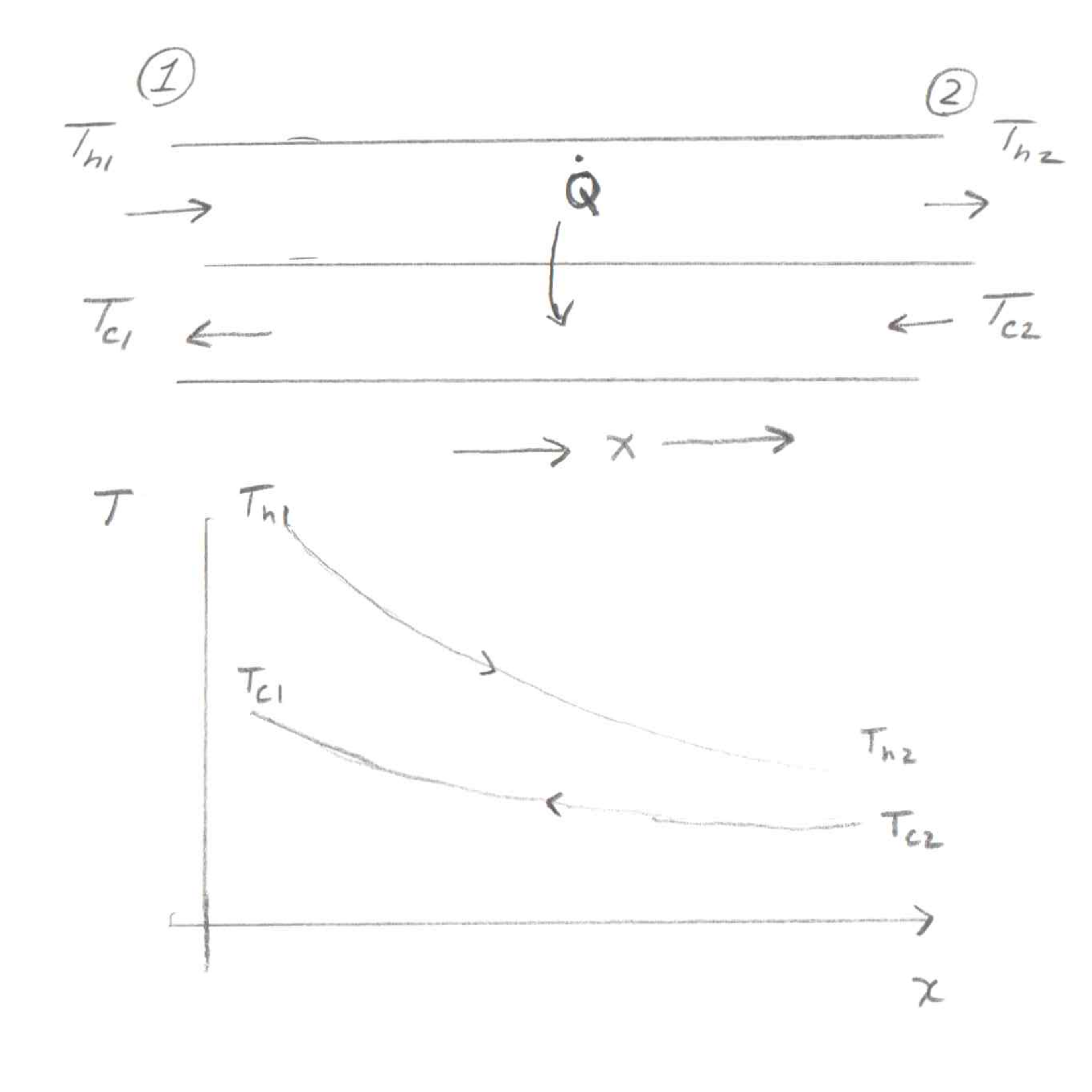
So here's a diagram of the setup. We've got two fluids, one hot and one cold, flowing in opposite directions. I've drawn the hot fluid on top going to the right and the cold fluid on the bottom going to the left. This is one dimensional, and the dimension is \(x\), going to the right.
The basic essence of this derivation is that we have two energy balances (equations that look like \(Q=mcΔT\)) and a form of the heat transfer rate (like \(Q=UAΔT\)).
For a simple fluid experiencing only heat transfer, we have:
\[ \dot{Q} = \dot{m} c_p \left(T_{out} - T_{in} \right) \]
However, I'm going to write it a little differently, using \(x\) as our variable representing 1-D distance along the heat exchanger. Important to note here is that \(T\) is a function of \(x\) (I'm going to color this function syntax red like this for clarity: \(T{\color{red}(x)}\)).
\[ \dot{Q} = \dot{m} c_p \left(T{\color{red}(x + Δx)} - T{\color{red}(x)}\right) \]
For reasons that will make more sense later, I'm going to divide both sides by that \(Δx\).
\[ \frac{\dot{Q}}{Δx} = \dot{m} c_p \left(\frac{T{\color{red} (x + Δx) } - T{\color{red}(x)}}{Δx}\right) \]
Now, If you take the limit as \(Δx\) goes to zero, you get the definition of the derivative of \(T\) with respect to \(x\) in that parenthesis.
\[ \lim_{Δx \to 0} \frac{\dot{Q}}{Δx} = \dot{m} c_p \frac{dT}{dx} \]
That \(\lim_{Δx \to 0} \dot{Q}/Δx\) is a little strange, but in the other derivations I've seen, most just call it the "differential" of \(\dot{Q}\). But we're going to want to give it a name, so I'm going to call it \(\delta{} \dot{Q}\).
\[ \delta \dot{Q} = \dot{m} c_p \frac{dT}{dx} \]
Let's also replace the \(\dot{m} c_p\) with \(C\), which is the heat capacity rate of the fluid. We have this formula for both the hot and cold fluids, so we'll subscript them with \(h\) and \(c\).
\begin{equation}\label{eq:eb} \delta \dot{Q} = C_h \frac{dT_h}{dx} = C_c \frac{dT_c}{dx} \end{equation}
At this point, I've not given any focus to the sign of the heat transfer rate. It may seem strange at first, but I'm going to add a negative to the RHS of each of these. Once you look at a plot of the temperature profiles, it will make more sense.
As you go from left to right (increasing \(x\)) on the plot, both temperatures are decreasing. This means that the \(dT/dx\) is negative for both fluids. We'd prefer to deal with a positive heat transfer rate everywhere, so this means that we need to add a negative sign to both equations.
\[ \delta \dot{Q} = -C_h \frac{dT_h}{dx} = -C_c \frac{dT_c}{dx} \]
Now we can look at another way to calculate the heat transfer rate. This is simply using the definition of the overall heat transfer coefficient \(U\). I'm using \(W\) to represent some constant "width" of the heat exchanger, such that the cross-sectional area is \(A = W Δx\).
I'm also going to assume some length that this heat transfer is happening over, \(x_{0}\) to \(x_{0} + \Delta x\). The \(UA\) value is going to be multiplied by the average temperature difference between the two fluids (using the calculus definition of average).
\[ \dot{Q} = U W Δx \int_{x_{0}}^{x_{0} + \Delta x} \frac{\left(T_{h} {\color{red}(x)}- T_{c}{\color{red}(x)}\right)}{ \Delta x} \]
Again, we can divide both sides by \(Δx\).
\[ \frac{\dot{Q}}{Δx} = U W \int_{x_{0}}^{x_{0} + \Delta x} \frac{\left(T_{h} {\color{red}(x)}- T_{c}{\color{red}(x)}\right)}{ \Delta x} \]
But before we take the limit as \(Δx\) goes to zero, let's evaluate that integral. I'm going to use \(T^{*}\) to represent some antiderivative of \(T\).
\[ \frac{\dot{Q}}{Δx} = U W \left( \frac{T^{*}_{h} {\color{red}(x_{0} + \Delta x)} - T^{*}_{h} {\color{red}(x_{0})}}{Δx} - \frac{T^{*}_{c} {\color{red}(x_{0} + \Delta x)} - T^{*}_{c} {\color{red}(x_{0})}}{Δx}\right) \]
Now let's take that limit. We can use our definition of \(\delta \dot{Q}\) to replace the left side. The temperature differences are again in the form of the definition of the derivative.
\[ \delta \dot{Q} = U W \left( \frac{dT^{*}_{h}}{dx} - \frac{dT^{*}_{c}}{dx} \right) \]
But \(T^{*}\) was assumed to be an antiderivative of \(T\), so we can replace the derivatives with the original functions.
\begin{equation}\label{eq:deltaq} \delta \dot{Q} = U W \left(T_{h}{\color{red}(x)}- T_{c}{\color{red}(x)}\right) \end{equation}
(Ok, some of you probably didn't need that level of detail to accept the above equation at face value. But I did.)
Let's rearrange the energy balance equations, to get a differential of the temperature differences. \(\def\dq{\delta \dot{Q}}\)
\[ \frac{dT_h}{dx} - \frac{dT_c}{dx} = \left( \frac{1}{-C_h} - \frac{1}{-C_c} \right) \dq \]
Differentiation is a linear operator, this means that the difference of derivatives is equal to the derivative of the difference. Also moving some things around on the RHS to deal with the double negative. \(\def\Cdiff{\left( \frac{1}{C_c} - \frac{1}{C_h} \right)}\)
\[ \frac{d}{dx} \left(T_h - T_c \right) = \left( \frac{1}{C_c} - \frac{1}{C_h} \right) \dq \]
We can now substitute \eqref{eq:deltaq} for \(\dq\) (dropping the function syntax).
\[ \frac{d}{dx} \left(T_h - T_c \right) = \Cdiff U W \left(T_{h} - T_{c}\right) \]
Let's move all the temperature differences to the LHS.
\[ \frac{\frac{d}{dx} \left(T_h - T_c \right)}{T_h - T_c} = \Cdiff U W \]
I'm going to define a new variable for the temperature difference, \(D\) (standing for difference).
\[ D = T_h - T_c \] \[ \frac{1}{D} \frac{dD}{dx} = \Cdiff U W \]
Integrating both sides with respect to \(x\), we get:
\[ \int_1^2 \frac{1}{D} \frac{dD}{dx} dx = \int_1^2 \Cdiff U W dx \] \[ \left.\ln D \right|_1^2 = \Cdiff U W L \] \[ \ln D_2 - \ln D_1 = \ln \frac{D_2}{D_1} = \Cdiff U A \]
Multiply and divide RHS by \(-C_h\).\[ \ln \frac{D_2}{D_1} = \left(1 - \frac{C_h}{C_c} \right) \frac{UA}{-C_h} \] \[ \ln \frac{D_2}{D_1} = -N_{tu} \left( 1 - \frac{C_h}{C_c} \right) \]
Let's bring back the temperatures by replacing the definition of \(D\).
\begin{equation}\label{eq:ln} \ln \frac{T_{h2} - T_{c2}}{T_{h1} - T_{c1}} = -N_{tu} \left( 1 - \frac{C_h}{C_c} \right) \end{equation}
Note that we replaced \(\frac{UA}{C_h}\) with \(N_{tu}\). \(N_{tu}\) is defined as \(UA/C_{min}\), where \(C_{min}\) is the minimum heat capacity rate of the fluids.
At this point, the hard part is done. What remains is algebraic manipulation with the definition of effectiveness.
The eventual goal is to get this in terms of effectiveness, ε, removing all the temperatures. The original Kays and London text with this derivation relies on a geometric interpretation that is really nice. However, I'm going to show a different line of algebraic thought that also works.
First we need to define effectiveness. We have implicitly assumed that \(C_{h} < C_{c}\), meaning that the hot flow has a lower heat capacity rate. Whichever fluid has the lower heat capacity rate will have the maximum temperature difference, with the largest possible difference being the difference between the inlet hot temperature and the inlet cold temperature. So effectiveness is defined as the ratio of the actual temperature difference to the maximum possible temperature difference.
\begin{equation}\label{eq:eff} ε = \frac{T_{h1} - T_{h2}}{T_{h1} - T_{c2}} \end{equation}
In \eqref{eq:ln}, we have differences in temperatures at the same end, 1's with 1's and 2's with 2's. Our effectiveness definition has differences in temperatures at opposite ends, 1's with 2's. The other key insight here is that we know the temperatures differences from end 1 to end 2 are proportional, based on \eqref{eq:eb}. Using \eqref{eq:eb}, we can write:
\[ \frac{dT_h}{dT_c} = \frac{C_c}{C_h} = \frac{T_{h1} - T_{h2}}{T_{c1} - T_{c2}} \]
Looking at the numerator of \eqref{eq:ln}, we have temperatures at end 2 (\(T_{h2} - T_{c2}\)). The simplest way to get the temperature differences between ends 1 and 2 is to add and subtract one of the temperatures at end 1, either \(T_{h1}\) or \(T_{c1}\). Arbitrarily, let's try adding and subtracting \(T_{h1}\).
\[ T_{h2} - T_{c2} = T_{h2} - T_{c2} + T_{h1} - T_{h1} = \left( T_{h1} - T_{c2} \right) - \left(T_{h1} - T_{h2}\right) \]
This is good because the terms \(\left( T_{h1} - T_{c2} \right)\) and \(\left(T_{h1} - T_{h2}\right)\) are both in the definition of effectiveness \eqref{eq:eff}.
Doing a similar thing for the bottom, but this time adding and subtracting \(T_{c1}\).\[ T_{h1} - T_{c1} = T_{h1} - T_{c1} + T_{c2} - T_{c2} = \left( T_{h1} - T_{c2} \right) - \left(T_{c1} - T_{c2}\right) \]
As a reminder, we are trying to simply the fraction on the LHS of \eqref{eq:ln}.\[ \frac{T_{h2} - T_{c2}}{T_{h1} - T_{c1}} = \frac{\left( T_{h1} - T_{c2} \right) - \left(T_{h1} - T_{h2}\right)}{\left( T_{h1} - T_{c2} \right) - \left(T_{c1} - T_{c2}\right)} \]
Hopefully you can see that by dividing the top and bottom by \(\left( T_{h1} - T_{c2} \right)\), we are going to cancel the first terms in the numerator and denominator and get 1's, and then we'll get an effectiveness term right away on the top.\[ \frac{\left( T_{h1} - T_{c2} \right) - \left(T_{h1} - T_{h2}\right)}{\left( T_{h1} - T_{c2} \right) - \left(T_{c1} - T_{c2}\right)} = \frac{ \frac{\left( T_{h1} - T_{c2} \right) - \left(T_{h1} - T_{h2}\right)}{ \left( T_{h1} - T_{c2} \right) } }{ \frac{\left( T_{h1} - T_{c2} \right) - \left(T_{c1} - T_{c2}\right)}{ \left( T_{h1} - T_{c2} \right) } } = \frac{1 - ε}{1 - \frac{ T_{c1} - T_{c2}}{ T_{h1} - T_{c2} } } \]
We're close now. If that \(T_{c1} - T_{c2}\) term just had \(h\)'s instead, we'd have another effectiveness term. Fortunately, we have a conversion factor for that, \(\frac{C_c}{C_h}\).
Replace \(T_{c1} - T_{c2}\) with \(\frac{C_h}{C_c} \left( T_{h1} - T_{h2} \right)\), and we now have an expression with no temperatures.
\[ \frac{T_{h2} - T_{c2}}{T_{h1} - T_{c1}} = \frac{1 - ε}{1 - \frac{C_h}{C_c} ε} \]
Now it's just algebra time - let's substitute this back into \eqref{eq:ln} and solve for \(ε\).
\[ \ln \left( \frac{1 - ε}{1 - \frac{C_h}{C_c} ε} \right) = -N_{tu} \left( 1 - \frac{C_h}{C_c} \right) \] \[ \left( \frac{1 - ε}{1 - \frac{C_h}{C_c} ε} \right) = e^{-N_{tu} \left( 1 - \frac{C_h}{C_c} \right) } \] \[ 1 - ε = \left( 1 - \frac{C_h}{C_c} ε \right) e^{-N_{tu} \left( 1 - \frac{C_h}{C_c} \right) } \] \[ 1 - ε = e^{-N_{tu} \left( 1 - \frac{C_h}{C_c} \right) } - \frac{C_h}{C_c} ε e^{-N_{tu} \left( 1 - \frac{C_h}{C_c} \right) } \] \[ 1 - e^{-N_{tu} \left( 1 - \frac{C_h}{C_c} \right) } = ε \left( 1 - \frac{C_h}{C_c} e^{-N_{tu} \left( 1 - \frac{C_h}{C_c} \right) } \right) \] \[ ε = \frac{1 - e^{-N_{tu} \left( 1 - \frac{C_h}{C_c} \right) }}{1 - \frac{C_h}{C_c} e^{-N_{tu} \left( 1 - \frac{C_h}{C_c} \right) } } \]
Now, since our assumption throughout was that \(C_h \lt C_c\), we can account for that here, and we get the final result that you'll see in your heat transfer textbooks.
\[ \epsilon = \frac{1 - e^{-NTU(1-\frac{C_{min}}{C_{max}})}}{1 - \frac{C_{min}}{C_{max}} e^{-NTU(1 - \frac{C_min{}}{C_{max}} )}} \]